This article walks through an example of creating a transaction study using the actxps package. Unlike a termination study, transaction studies track events that can occur multiple times over the life of a policy. Often, transactions are expected to reoccur; for example, the utilization of a guaranteed income stream.
Key questions to answer in a transaction study are:
- What types of transactions occurred?
- What is the count, amount, and average size of observed transactions?
- What percentage of policies have transactions each exposure period?
- How do transactions compare to expectations?
- What is the rate of transaction amounts as a percentage of another value?
The example below walks through preparing data by adding transaction
information to a data frame with exposure-level records using the
add_transactions() function. Next, study results are
summarized using the trx_stats() function.
Simulated transaction and account value data
In this example, we’ll be using the census_dat,
withdrawals, and account_vals data sets. Each
data set is based on a theoretical block of deferred annuity business
with a guaranteed lifetime income benefit.
-
census_datcontains census-level information with one row per policy -
withdrawalscontains withdrawal transactions. There are 2 types of transactions in the data: “Base” (ordinary withdrawals) and “Rider” (guaranteed income payments). -
account_valscontains historical account values on policy anniversaries. This data will be used to calculate withdrawal rates as a percentage of account values.
The add_transactions() function
The add_transactions() function attaches transactions to
a data frame with exposure-level records. This data frame must have the
class exposed_df. For our example, we first need to convert
census_dat into exposure records using the
expose() function.1 This example will use policy year
exposures.
library(actxps)
#>
#> Attaching package: 'actxps'
#> The following object is masked from 'package:stats':
#>
#>     filter
library(dplyr)
#>
#> Attaching package: 'dplyr'
#> The following objects are masked from 'package:stats':
#>
#>     filter, lag
#> The following objects are masked from 'package:base':
#>
#>     intersect, setdiff, setequal, union

exposed_data <- expose_py(census_dat, "2019-12-31", target_status = "Surrender")
exposed_data
#>
#> ── Exposure data ──
#>
#> • Exposure type: policy_year
#> • Target status: Surrender
#> • Study range: 1900-01-01 to 2019-12-31
#>
#> # A tibble: 141,252 × 15
#>    pol_num status issue_date inc_guar qual    age product gender wd_age premium
#>      <int> <fct>  <date>     <lgl>    <lgl> <int> <fct>   <fct>   <int>   <dbl>
#>  1       1 Active 2014-12-17 TRUE     FALSE    56 b       F          77     370
#>  2       1 Active 2014-12-17 TRUE     FALSE    56 b       F          77     370
#>  3       1 Active 2014-12-17 TRUE     FALSE    56 b       F          77     370
#>  4       1 Active 2014-12-17 TRUE     FALSE    56 b       F          77     370
#>  5       1 Active 2014-12-17 TRUE     FALSE    56 b       F          77     370
#>  6       1 Active 2014-12-17 TRUE     FALSE    56 b       F          77     370
#>  7       2 Active 2007-09-24 FALSE    FALSE    71 a       F          71     708
#>  8       2 Active 2007-09-24 FALSE    FALSE    71 a       F          71     708
#>  9       2 Active 2007-09-24 FALSE    FALSE    71 a       F          71     708
#> 10       2 Active 2007-09-24 FALSE    FALSE    71 a       F          71     708
#> # ℹ 141,242 more rows
#> # ℹ 5 more variables: term_date <date>, pol_yr <int>, pol_date_yr <date>,
#> #   pol_date_yr_end <date>, exposure <dbl>
The withdrawals data has 4 columns that are required for
attaching transactions:
-
pol_num: policy number -
trx_date: transaction date -
trx_type: transaction type -
trx_amt: transaction amount
withdrawals
#> # A tibble: 160,130 × 4
#>    pol_num trx_date   trx_type trx_amt
#>      <int> <date>     <fct>      <dbl>
#>  1       2 2007-10-05 Base          25
#>  2       2 2009-07-30 Base          12
#>  3       2 2010-02-22 Base           7
#>  4       2 2010-12-30 Base          52
#>  5       2 2012-05-07 Base          41
#>  6       2 2013-03-15 Base           1
#>  7       2 2013-12-06 Base           2
#>  8       2 2015-05-18 Base           2
#>  9       2 2016-05-10 Base           8
#> 10       2 2017-01-08 Base           2
#> # ℹ 160,120 more rows
The grain of this data is one row per policy per transaction. The expectation is that the number of records in the transaction data will not match the number of rows in the exposure data. That is because policies could have zero or several transactions in a given exposure period.
The add_transactions() function uses a non-equivalent
join to associate each transaction with a policy number and a date
interval found in the exposure data. Then, transaction counts and
amounts are summarized such that there is one row per exposure period.
In the event there are multiple transaction types found in the data,
separate columns are created for each transaction type.
Using our example, we pass both the exposure and withdrawals data to
add_transactions(). The resulting data has the same number
of rows as original exposure data and 4 new columns:
-
trx_amt_Base: the sum of “Base” withdrawal transactions -
trx_amt_Rider: the sum of “Rider” withdrawal transactions -
trx_n_Base: the number of “Base” withdrawal transactions -
trx_n_Rider: the number of “Rider” withdrawal transactions
exposed_trx <- add_transactions(exposed_data, withdrawals)
glimpse(exposed_trx)
#> Rows: 141,252
#> Columns: 19
#> $ pol_num         <int> 1, 1, 1, 1, 1, 1, 2, 2, 2, 2, 2, 2, 2, 2, 2, 2, 2, 2, …
#> $ status          <fct> Active, Active, Active, Active, Active, Active, Active…
#> $ issue_date      <date> 2014-12-17, 2014-12-17, 2014-12-17, 2014-12-17, 2014-…
#> $ inc_guar        <lgl> TRUE, TRUE, TRUE, TRUE, TRUE, TRUE, FALSE, FALSE, FALS…
#> $ qual            <lgl> FALSE, FALSE, FALSE, FALSE, FALSE, FALSE, FALSE, FALSE…
#> $ age             <int> 56, 56, 56, 56, 56, 56, 71, 71, 71, 71, 71, 71, 71, 71…
#> $ product         <fct> b, b, b, b, b, b, a, a, a, a, a, a, a, a, a, a, a, a, …
#> $ gender          <fct> F, F, F, F, F, F, F, F, F, F, F, F, F, F, F, F, F, F, …
#> $ wd_age          <int> 77, 77, 77, 77, 77, 77, 71, 71, 71, 71, 71, 71, 71, 71…
#> $ premium         <dbl> 370, 370, 370, 370, 370, 370, 708, 708, 708, 708, 708,…
#> $ term_date       <date> NA, NA, NA, NA, NA, NA, NA, NA, NA, NA, NA, NA, NA, N…
#> $ pol_yr          <int> 1, 2, 3, 4, 5, 6, 1, 2, 3, 4, 5, 6, 7, 8, 9, 10, 11, 1…
#> $ pol_date_yr     <date> 2014-12-17, 2015-12-17, 2016-12-17, 2017-12-17, 2018-…
#> $ pol_date_yr_end <date> 2015-12-16, 2016-12-16, 2017-12-16, 2018-12-16, 2019-…
#> $ exposure        <dbl> 1.00000000, 1.00000000, 1.00000000, 1.00000000, 1.0000…
#> $ trx_amt_Base    <dbl> 0, 0, 0, 0, 0, 0, 25, 12, 7, 52, 41, 1, 2, 2, 8, 2, 44…
#> $ trx_amt_Rider   <dbl> 0, 0, 0, 0, 0, 0, 0, 0, 0, 0, 0, 0, 0, 0, 0, 0, 0, 0, …
#> $ trx_n_Base      <dbl> 0, 0, 0, 0, 0, 0, 1, 1, 1, 1, 1, 1, 1, 1, 1, 1, 1, 1, …
#> $ trx_n_Rider     <dbl> 0, 0, 0, 0, 0, 0, 0, 0, 0, 0, 0, 0, 0, 0, 0, 0, 0, 0, …
If we print exposed_trx, we can see that it is still an
exposed_df object, but now it has an additional attribute
for transaction types that have been attached.
exposed_trx
#>
#> ── Exposure data ──
#>
#> • Exposure type: policy_year
#> • Target status: Surrender
#> • Study range: 1900-01-01 to 2019-12-31
#> • Transaction types: Base and Rider
#>
#> # A tibble: 141,252 × 19
#>    pol_num status issue_date inc_guar qual    age product gender wd_age premium
#>      <int> <fct>  <date>     <lgl>    <lgl> <int> <fct>   <fct>   <int>   <dbl>
#>  1       1 Active 2014-12-17 TRUE     FALSE    56 b       F          77     370
#>  2       1 Active 2014-12-17 TRUE     FALSE    56 b       F          77     370
#>  3       1 Active 2014-12-17 TRUE     FALSE    56 b       F          77     370
#>  4       1 Active 2014-12-17 TRUE     FALSE    56 b       F          77     370
#>  5       1 Active 2014-12-17 TRUE     FALSE    56 b       F          77     370
#>  6       1 Active 2014-12-17 TRUE     FALSE    56 b       F          77     370
#>  7       2 Active 2007-09-24 FALSE    FALSE    71 a       F          71     708
#>  8       2 Active 2007-09-24 FALSE    FALSE    71 a       F          71     708
#>  9       2 Active 2007-09-24 FALSE    FALSE    71 a       F          71     708
#> 10       2 Active 2007-09-24 FALSE    FALSE    71 a       F          71     708
#> # ℹ 141,242 more rows
#> # ℹ 9 more variables: term_date <date>, pol_yr <int>, pol_date_yr <date>,
#> #   pol_date_yr_end <date>, exposure <dbl>, trx_amt_Base <dbl>,
#> #   trx_amt_Rider <dbl>, trx_n_Base <dbl>, trx_n_Rider <dbl>
The trx_stats() function
The actxps package’s workhorse function for summarizing transaction
experience is trx_stats(). This function returns a
trx_df object, which is a type of data frame containing
additional attributes about the transaction study.
At a minimum, a trx_df includes the following for each
transaction type (trx_type):
- The number of transactions (
trx_n) - The number of exposure periods with a transaction
(
trx_flag) - The sum of transactions (
trx_amt) - The total exposure (
exposure) - The average transaction amount when a transaction occurs
(
avg_trx) - The average transaction amount across all records
(
avg_all) - The transaction frequency when a transaction occurs
(
trx_freq = trx_n / trx_flag) - The transaction utilization
(
trx_util = trx_flag / exposure)
Optionally, a trx_df can also include:
- Any grouping variables attached to the input data
- Transaction amounts as a percentage of another value when a
transaction occurs (
pct_of_*_w_trx) - Transaction amounts as a percentage of another value across all
records (
pct_of_*_all)
To use trx_stats(), we simply need to pass it an
exposed_df object with transactions attached.2
trx_stats(exposed_trx)
#>
#> ── Transaction study results ──
#>
#> • Study range: 1900-01-01 to 2019-12-31
#> • Transaction types: Base and Rider
#>
#> # A tibble: 2 × 9
#>   trx_type trx_n trx_flag trx_amt exposure avg_trx avg_all trx_freq trx_util
#>   <chr>    <dbl>    <int>   <dbl>    <dbl>   <dbl>   <dbl>    <dbl>    <dbl>
#> 1 Base     60500    28224 1093899   124173    38.8    8.81     2.14    0.227
#> 2 Rider    77321    35941 2842729   124173    79.1   22.9      2.15    0.289
The results show us that we specified no groups, which is why the output data contains a single row for each transaction type.
Grouped data
If the data frame passed into trx_stats() is grouped
using dplyr::group_by(), the resulting output will contain
one record for each transaction type for each unique group.
In the following, exposed_trx is grouped by the presence
of an income guarantee (inc_guar) before being passed to
trx_stats(). This results in four rows because we have two
types of transactions and two distinct values of
inc_guar.
exposed_trx |>
  group_by(inc_guar) |>
  trx_stats()
#>
#> ── Transaction study results ──
#>
#> • Groups: inc_guar
#> • Study range: 1900-01-01 to 2019-12-31
#> • Transaction types: Base and Rider
#>
#> # A tibble: 4 × 10
#>   inc_guar trx_type trx_n trx_flag trx_amt exposure avg_trx avg_all trx_freq
#>   <lgl>    <chr>    <dbl>    <int>   <dbl>    <dbl>   <dbl>   <dbl>    <dbl>
#> 1 FALSE    Base     52939    24703  952629    48938    38.6   19.5      2.14
#> 2 FALSE    Rider        0        0       0    48938   NaN      0      NaN
#> 3 TRUE     Base      7561     3521  141270    75235    40.1    1.88     2.15
#> 4 TRUE     Rider    77321    35941 2842729    75235    79.1   37.8      2.15
#> # ℹ 1 more variable: trx_util <dbl>
Multiple grouping variables are allowed. Below, policy year
(pol_yr) is added as a second grouping variable.
exposed_trx |>
  group_by(pol_yr, inc_guar) |>
  trx_stats()
#>
#> ── Transaction study results ──
#>
#> • Groups: pol_yr and inc_guar
#> • Study range: 1900-01-01 to 2019-12-31
#> • Transaction types: Base and Rider
#>
#> # A tibble: 60 × 11
#>    pol_yr inc_guar trx_type trx_n trx_flag trx_amt exposure avg_trx avg_all
#>     <int> <lgl>    <chr>    <dbl>    <int>   <dbl>    <dbl>   <dbl>   <dbl>
#>  1      1 FALSE    Base      6077     2881   98287     7435    34.1   13.2
#>  2      1 FALSE    Rider        0        0       0     7435   NaN      0
#>  3      1 TRUE     Base      1370      633   21590    11106    34.1    1.94
#>  4      1 TRUE     Rider     8077     3778  265312    11106    70.2   23.9
#>  5      2 FALSE    Base      6091     2863   98413     6813    34.4   14.4
#>  6      2 FALSE    Rider        0        0       0     6813   NaN      0
#>  7      2 TRUE     Base      1183      559   18554    10158    33.2    1.83
#>  8      2 TRUE     Rider     8232     3834  288114    10158    75.1   28.4
#>  9      3 FALSE    Base      6016     2813   97285     6176    34.6   15.8
#> 10      3 FALSE    Rider        0        0       0     6176   NaN      0
#> # ℹ 50 more rows
#> # ℹ 2 more variables: trx_freq <dbl>, trx_util <dbl>
Expressing transactions as a percentage of another value
In a transaction study, we often want to express transaction amounts as a percentage of another value. For example, in a withdrawal study, withdrawal amounts divided by account values provides a withdrawal rate. In a study of benefit utilization, transactions can be divided by a maximum benefit amount to derive a benefit utilization rate. In addition, actual-to-expected rates can be calculated by dividing transactions by expected values.
If column names are passed to the percent_of argument of
trx_stats(), the output will contain 4 additional columns
for each “percent of” variable:
- The sum of each “percent of” variable
- The sum of each “percent of” variable when a transaction occurs.
These columns include the suffix
_w_trx. - Transaction amounts divided by each “percent of” variable
(
pct_of_{*}_all) - Transaction amounts divided by each “percent of” variable when a
transaction occurs (
pct_of_{*}_w_trx)
For our example, let’s assume we’re interested in examining
withdrawal transactions as a percentage of account values, which are
available in the account_vals data frame in the column
av_anniv.
# attach account values data
exposed_trx_w_av <- exposed_trx |>
  left_join(account_vals, by = c("pol_num", "pol_date_yr"))

trx_res <- exposed_trx_w_av |>
  group_by(pol_yr, inc_guar) |>
  trx_stats(percent_of = "av_anniv")

glimpse(trx_res)
#> Rows: 60
#> Columns: 15
#> $ pol_yr                <int> 1, 1, 1, 1, 2, 2, 2, 2, 3, 3, 3, 3, 4, 4, 4, 4, …
#> $ inc_guar              <lgl> FALSE, FALSE, TRUE, TRUE, FALSE, FALSE, TRUE, TR…
#> $ trx_type              <chr> "Base", "Rider", "Base", "Rider", "Base", "Rider…
#> $ trx_n                 <dbl> 6077, 0, 1370, 8077, 6091, 0, 1183, 8232, 6016, …
#> $ trx_flag              <int> 2881, 0, 633, 3778, 2863, 0, 559, 3834, 2813, 0,…
#> $ trx_amt               <dbl> 98287, 0, 21590, 265312, 98413, 0, 18554, 288114…
#> $ exposure              <dbl> 7435, 7435, 11106, 11106, 6813, 6813, 10158, 101…
#> $ avg_trx               <dbl> 34.11558, NaN, 34.10742, 70.22552, 34.37408, NaN…
#> $ avg_all               <dbl> 13.219502, 0.000000, 1.943994, 23.889069, 14.444…
#> $ trx_freq              <dbl> 2.109337, NaN, 2.164297, 2.137904, 2.127489, NaN…
#> $ trx_util              <dbl> 0.38749159, 0.00000000, 0.05699622, 0.34017648, …
#> $ av_anniv_w_trx        <dbl> 3875306, 0, 865046, 4982082, 3909786, 0, 797932,…
#> $ av_anniv              <dbl> 9686914, 9686914, 14679001, 14679001, 9218561, 9…
#> $ pct_of_av_anniv_w_trx <dbl> 0.02536238, NaN, 0.02495821, 0.05325324, 0.02517…
#> $ pct_of_av_anniv_all   <dbl> 0.010146369, 0.000000000, 0.001470809, 0.0180742…
Confidence intervals
If conf_int is set to TRUE,
trx_stats() will produce lower and upper confidence
interval limits for the observed utilization rate. Confidence intervals
are constructed assuming a binomial distribution.
exposed_trx |>
  group_by(pol_yr) |>
  trx_stats(conf_int = TRUE) |>
  select(pol_yr, trx_util, trx_util_lower, trx_util_upper)
#>
#> ── Transaction study results ──
#>
#> • Groups: pol_yr
#> • Study range: 1900-01-01 to 2019-12-31
#> • Transaction types: Base and Rider
#>
#> # A tibble: 30 × 4
#>    pol_yr trx_util trx_util_lower trx_util_upper
#>     <int>    <dbl>          <dbl>          <dbl>
#>  1      1    0.190          0.184          0.195
#>  2      1    0.204          0.198          0.210
#>  3      2    0.202          0.196          0.208
#>  4      2    0.226          0.220          0.232
#>  5      3    0.215          0.208          0.221
#>  6      3    0.248          0.241          0.255
#>  7      4    0.223          0.216          0.230
#>  8      4    0.269          0.262          0.277
#>  9      5    0.233          0.225          0.240
#> 10      5    0.288          0.280          0.296
#> # ℹ 20 more rows
The default confidence level is 95%. This can be changed using the
conf_level argument. Below, tighter confidence intervals
are constructed by decreasing the confidence level to 90%.
exposed_trx |>
  group_by(pol_yr) |>
  trx_stats(conf_int = TRUE, conf_level = 0.9) |>
  select(pol_yr, trx_util, trx_util_lower, trx_util_upper)
#>
#> ── Transaction study results ──
#>
#> • Groups: pol_yr
#> • Study range: 1900-01-01 to 2019-12-31
#> • Transaction types: Base and Rider
#>
#> # A tibble: 30 × 4
#>    pol_yr trx_util trx_util_lower trx_util_upper
#>     <int>    <dbl>          <dbl>          <dbl>
#>  1      1    0.190          0.185          0.194
#>  2      1    0.204          0.199          0.209
#>  3      2    0.202          0.197          0.207
#>  4      2    0.226          0.221          0.231
#>  5      3    0.215          0.209          0.220
#>  6      3    0.248          0.242          0.254
#>  7      4    0.223          0.218          0.229
#>  8      4    0.269          0.263          0.276
#>  9      5    0.233          0.226          0.239
#> 10      5    0.288          0.281          0.295
#> # ℹ 20 more rows
If any column names are passed to percent_of,
trx_stats() will produce additional confidence
intervals:
- Intervals for transactions as a percentage of another column when
transactions occur (
pct_of_{*}_w_trx) are constructed using a normal distribution. - Intervals for transactions as a percentage of another column
regardless of transaction utilization (
pct_of_{*}_all) are calculated assuming that the aggregate distribution is normal with a mean equal to observed transactions and a variance equal to:
Where S is the aggregate
transactions random variable, X is an individual
transaction amount assumed to follow a normal distribution, and
N is a binomial random variable for transaction
utilization.
exposed_trx_w_av |>
  group_by(pol_yr) |>
  trx_stats(conf_int = TRUE, percent_of = "av_anniv") |>
  select(pol_yr, starts_with("pct_of")) |>
  glimpse()
#> Rows: 30
#> Columns: 7
#> $ pol_yr                      <int> 1, 1, 2, 2, 3, 3, 4, 4, 5, 5, 6, 6, 7, 7, …
#> $ pct_of_av_anniv_w_trx       <dbl> 0.02528863, 0.05325324, 0.02484580, 0.0573…
#> $ pct_of_av_anniv_all         <dbl> 0.004919864, 0.010888653, 0.005082440, 0.0…
#> $ pct_of_av_anniv_w_trx_lower <dbl> 0.02401960, 0.05078956, 0.02362583, 0.0544…
#> $ pct_of_av_anniv_w_trx_upper <dbl> 0.02655765, 0.05571692, 0.02606577, 0.0602…
#> $ pct_of_av_anniv_all_lower   <dbl> 0.004632812, 0.010297256, 0.004790158, 0.0…
#> $ pct_of_av_anniv_all_upper   <dbl> 0.005206917, 0.011480050, 0.005374723, 0.0…
autoplot() and autotable()
The autoplot() and autotable() functions
create visualizations and summary tables from trx_df
objects. See vignette("visualizations") for full details on
these functions.
library(ggplot2)

trx_res |>
  # remove periods with zero transactions
  filter(trx_n > 0) |>
  autoplot(y = pct_of_av_anniv_w_trx)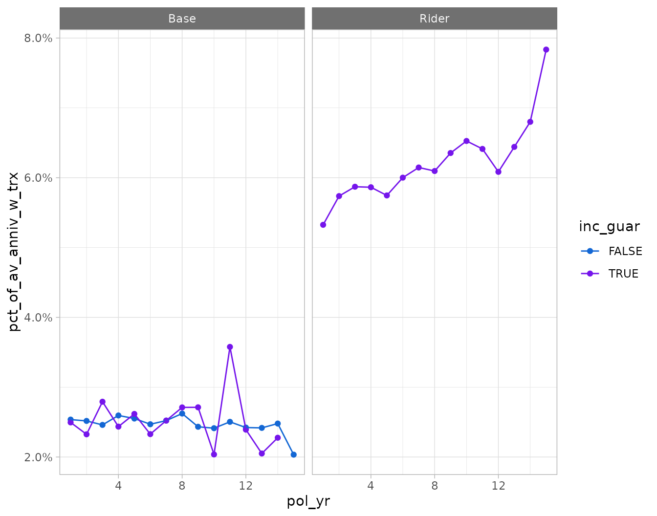
trx_res |>
  # remove periods with zero transactions
  filter(trx_n > 0) |>
  # first 10 rows showed for brevity
  head(10) |>
  autotable()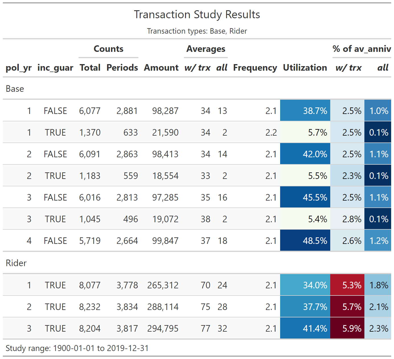
Miscellaneous
Selecting and combining transaction types
The trx_types argument of trx_stats()
selects a subset of transaction types that will appear in the
output.
trx_stats(exposed_trx, trx_types = "Base")
#>
#> ── Transaction study results ──
#>
#> • Study range: 1900-01-01 to 2019-12-31
#> • Transaction types: Base
#>
#> # A tibble: 1 × 9
#>   trx_type trx_n trx_flag trx_amt exposure avg_trx avg_all trx_freq trx_util
#>   <chr>    <dbl>    <int>   <dbl>    <dbl>   <dbl>   <dbl>    <dbl>    <dbl>
#> 1 Base     60500    28224 1093899   124173    38.8    8.81     2.14    0.227
If the combine_trx argument is set to TRUE,
all transaction types will be combined in a group called “All” in the
output.
trx_stats(exposed_trx, combine_trx = TRUE)
#>
#> ── Transaction study results ──
#>
#> • Study range: 1900-01-01 to 2019-12-31
#> • Transaction types: Base and Rider
#>
#> # A tibble: 1 × 9
#>   trx_type  trx_n trx_flag trx_amt exposure avg_trx avg_all trx_freq trx_util
#>   <chr>     <dbl>    <int>   <dbl>    <dbl>   <dbl>   <dbl>    <dbl>    <dbl>
#> 1 All      137821    64165 3936628   124173    61.4    31.7     2.15    0.517
Partial exposures are removed as a default
As a default, trx_stats() removes partial exposures
before summarizing results. This is done to avoid complexity associated
with a lopsided skew in the timing of transactions. For example, if
transactions can occur on a monthly basis or annually at the beginning
of each policy year, partial exposures may not be appropriate. If a
policy had an exposure of 0.5 years and was taking withdrawals annually
at the beginning of the year, an argument could be made that the
exposure should instead be 1 complete year. If the same policy was
expected to take withdrawals 9 months into the year, it’s not clear if
the exposure should be 0.5 years or 0.5 / 0.75 years. To override this
treatment, set the full_exposures_only argument to
FALSE.
trx_stats(exposed_trx, full_exposures_only = FALSE)
#>
#> ── Transaction study results ──
#>
#> • Study range: 1900-01-01 to 2019-12-31
#> • Transaction types: Base and Rider
#>
#> # A tibble: 2 × 9
#>   trx_type trx_n trx_flag trx_amt exposure avg_trx avg_all trx_freq trx_util
#>   <chr>    <dbl>    <int>   <dbl>    <dbl>   <dbl>   <dbl>    <dbl>    <dbl>
#> 1 Base     69430    32379 1271778  132634.    39.3    9.59     2.14    0.244
#> 2 Rider    90700    42139 3361541  132634.    79.8   25.3      2.15    0.318
Summary method
As noted above, the result of trx_stats() is a
trx_df object. If the summary() function is
applied to a trx_df object, the data will be summarized
again and return a higher level trx_df object.
If no additional arguments are passed, summary() returns
a single row of aggregate results for each transaction type.
summary(trx_res)
#>
#> ── Transaction study results ──
#>
#> • Study range: 1900-01-01 to 2019-12-31
#> • Transaction types: Base and Rider
#> • Transactions as % of: av_anniv
#>
#> # A tibble: 2 × 13
#>   trx_type trx_n trx_flag trx_amt exposure avg_trx avg_all trx_freq trx_util
#>   <chr>    <dbl>    <int>   <dbl>    <dbl>   <dbl>   <dbl>    <dbl>    <dbl>
#> 1 Base     60500    28224 1093899   124173    38.8    8.81     2.14    0.227
#> 2 Rider    77321    35941 2842729   124173    79.1   22.9      2.15    0.289
#> # ℹ 4 more variables: av_anniv_w_trx <dbl>, av_anniv <dbl>,
#> #   pct_of_av_anniv_w_trx <dbl>, pct_of_av_anniv_all <dbl>
If additional variable names are passed to the summary()
function, then the output will group the data by those variables. In our
example, if pol_yr is passed to summary(), the
output will contain one row per policy year for each transaction
type.
summary(trx_res, pol_yr)
#>
#> ── Transaction study results ──
#>
#> • Groups: pol_yr
#> • Study range: 1900-01-01 to 2019-12-31
#> • Transaction types: Base and Rider
#> • Transactions as % of: av_anniv
#>
#> # A tibble: 30 × 14
#>    pol_yr trx_type trx_n trx_flag trx_amt exposure avg_trx avg_all trx_freq
#>     <int> <chr>    <dbl>    <int>   <dbl>    <dbl>   <dbl>   <dbl>    <dbl>
#>  1      1 Base      7447     3514  119877    18541    34.1    6.47     2.12
#>  2      1 Rider     8077     3778  265312    18541    70.2   14.3      2.14
#>  3      2 Base      7274     3422  116967    16971    34.2    6.89     2.13
#>  4      2 Rider     8232     3834  288114    16971    75.1   17.0      2.15
#>  5      3 Base      7061     3309  116357    15397    35.2    7.56     2.13
#>  6      3 Rider     8204     3817  294795    15397    77.2   19.1      2.15
#>  7      4 Base      6596     3080  114987    13790    37.3    8.34     2.14
#>  8      4 Rider     7960     3715  283763    13790    76.4   20.6      2.14
#>  9      5 Base      6093     2847  109918    12234    38.6    8.98     2.14
#> 10      5 Rider     7536     3521  264939    12234    75.2   21.7      2.14
#> # ℹ 20 more rows
#> # ℹ 5 more variables: trx_util <dbl>, av_anniv_w_trx <dbl>, av_anniv <dbl>,
#> #   pct_of_av_anniv_w_trx <dbl>, pct_of_av_anniv_all <dbl>
Similarly, if inc_guar is passed to
summary(), the output will contain a row for each
transaction type and unique value in inc_guar.
summary(trx_res, inc_guar)
#>
#> ── Transaction study results ──
#>
#> • Groups: inc_guar
#> • Study range: 1900-01-01 to 2019-12-31
#> • Transaction types: Base and Rider
#> • Transactions as % of: av_anniv
#>
#> # A tibble: 4 × 14
#>   inc_guar trx_type trx_n trx_flag trx_amt exposure avg_trx avg_all trx_freq
#>   <lgl>    <chr>    <dbl>    <int>   <dbl>    <dbl>   <dbl>   <dbl>    <dbl>
#> 1 FALSE    Base     52939    24703  952629    48938    38.6   19.5      2.14
#> 2 FALSE    Rider        0        0       0    48938   NaN      0      NaN
#> 3 TRUE     Base      7561     3521  141270    75235    40.1    1.88     2.15
#> 4 TRUE     Rider    77321    35941 2842729    75235    79.1   37.8      2.15
#> # ℹ 5 more variables: trx_util <dbl>, av_anniv_w_trx <dbl>, av_anniv <dbl>,
#> #   pct_of_av_anniv_w_trx <dbl>, pct_of_av_anniv_all <dbl>
Column names
As a default, add_transactions() assumes the transaction
data frame (trx_data) uses the following naming
conventions:
- The policy number column is called
pol_num - The transaction date column is called
trx_date - The transaction type column is called
trx_type - The transaction amount column is called
trx_amt
These default names can be overridden using the
col_pol_num, col_trx_date,
col_trx_type, and col_trx_amt arguments.
For example, if the transaction type column was called
transaction_code in our data, we could write:
exposed_data |>
  add_transactions(withdrawals, col_trx_type = "transaction_code")
Similarly, trx_stats() assumes the input data uses the
name exposure for exposures. This default can be overridden
using the argument col_exposure.
Limitations
The trx_stats() function does not produce any
calculations related to the persistence of transactions from exposure
period to exposure period.