Getting started with actxps

This article is based on creating a termination study using sample data that comes with the actxps package. For information on transaction studies, see Transactions.

Simulated data set

The actxps package includes a Polars data frame containing simulated census data for a theoretical deferred annuity product with an optional guaranteed income rider. The grain of this data is one row per policy.

import actxps as xp
import numpy as np
import polars as pl

census_dat = xp.load_census_dat()
census_dat
shape: (20_000, 11)
pol_num status issue_date inc_guar qual age product gender wd_age premium term_date
i64 cat date bool bool i64 cat cat i64 f64 date
1 "Active" 2014-12-17 true false 56 "b" "F" 77 370.0 null
2 "Surrender" 2007-09-24 false false 71 "a" "F" 71 708.0 2019-03-08
3 "Active" 2012-10-06 false true 62 "b" "F" 63 466.0 null
4 "Surrender" 2005-06-27 true true 62 "c" "M" 62 485.0 2018-11-29
5 "Active" 2019-11-22 false false 62 "c" "F" 67 978.0 null
19996 "Active" 2014-08-11 true true 55 "b" "F" 75 3551.0 null
19997 "Surrender" 2006-11-20 false false 68 "c" "F" 77 336.0 2017-07-09
19998 "Surrender" 2017-02-20 true false 68 "c" "F" 68 1222.0 2018-08-03
19999 "Active" 2015-04-11 false true 67 "a" "M" 78 2138.0 null
20000 "Active" 2009-04-29 true true 72 "c" "M" 72 5751.0 null
Note

census_dat is a Polars data frame. Actxps functions accept both Polars and Pandas data frames. For speed and efficiency reasons, Polars is used internally for all data wrangling, so if a Pandas data frame is passed to an actxps function it will be converted to Polars. To convert a Polars data frame to Pandas the method DataFrame.to_pandas() is available.

The data includes 3 policy statuses: Active, Death, and Surrender.

status_counts = census_dat['status'].value_counts()
status_counts
shape: (3, 2)
status count
cat u32
"Active" 15212
"Death" 1816
"Surrender" 2972

Let’s assume we’re interested in calculating the probability of surrender over one policy year. We cannot simply calculate the proportion of policies in a surrendered status as this does not represent an annualized surrender rate.

# incorrect
status_counts.with_columns(pl.col('count') / pl.col('count').sum())
shape: (3, 2)
status count
cat f64
"Active" 0.7606
"Death" 0.0908
"Surrender" 0.1486

Creating exposed data

In order to calculate annual surrender rates, we need to break each policy into multiple records. There should be one row per policy per year.

The ExposedDF() class is used to perform this transformation.

exposed_data = xp.ExposedDF(census_dat, end_date="2019-12-31",
                            target_status="Surrender")

exposed_data
Exposure data

Exposure type: policy_year
Target status: Surrender
Study range: 1900-01-01 to 2019-12-31

shape: (141_252, 15)
┌─────────┬────────┬────────────┬──────────┬───┬────────┬─────────────┬─────────────────┬──────────┐
│ pol_num ┆ status ┆ issue_date ┆ inc_guar ┆ … ┆ pol_yr ┆ pol_date_yr ┆ pol_date_yr_end ┆ exposure │
│ ---     ┆ ---    ┆ ---        ┆ ---      ┆   ┆ ---    ┆ ---         ┆ ---             ┆ ---      │
│ i64     ┆ enum   ┆ date       ┆ bool     ┆   ┆ u32    ┆ date        ┆ date            ┆ f64      │
╞═════════╪════════╪════════════╪══════════╪═══╪════════╪═════════════╪═════════════════╪══════════╡
│ 1       ┆ Active ┆ 2014-12-17 ┆ true     ┆ … ┆ 1      ┆ 2014-12-17  ┆ 2015-12-16      ┆ 1.0      │
│ 1       ┆ Active ┆ 2014-12-17 ┆ true     ┆ … ┆ 2      ┆ 2015-12-17  ┆ 2016-12-16      ┆ 1.0      │
│ 1       ┆ Active ┆ 2014-12-17 ┆ true     ┆ … ┆ 3      ┆ 2016-12-17  ┆ 2017-12-16      ┆ 1.0      │
│ 1       ┆ Active ┆ 2014-12-17 ┆ true     ┆ … ┆ 4      ┆ 2017-12-17  ┆ 2018-12-16      ┆ 1.0      │
│ 1       ┆ Active ┆ 2014-12-17 ┆ true     ┆ … ┆ 5      ┆ 2018-12-17  ┆ 2019-12-16      ┆ 1.0      │
│ …       ┆ …      ┆ …          ┆ …        ┆ … ┆ …      ┆ …           ┆ …               ┆ …        │
│ 20000   ┆ Active ┆ 2009-04-29 ┆ true     ┆ … ┆ 7      ┆ 2015-04-29  ┆ 2016-04-28      ┆ 1.0      │
│ 20000   ┆ Active ┆ 2009-04-29 ┆ true     ┆ … ┆ 8      ┆ 2016-04-29  ┆ 2017-04-28      ┆ 1.0      │
│ 20000   ┆ Active ┆ 2009-04-29 ┆ true     ┆ … ┆ 9      ┆ 2017-04-29  ┆ 2018-04-28      ┆ 1.0      │
│ 20000   ┆ Active ┆ 2009-04-29 ┆ true     ┆ … ┆ 10     ┆ 2018-04-29  ┆ 2019-04-28      ┆ 1.0      │
│ 20000   ┆ Active ┆ 2009-04-29 ┆ true     ┆ … ┆ 11     ┆ 2019-04-29  ┆ 2020-04-28      ┆ 0.674863 │
└─────────┴────────┴────────────┴──────────┴───┴────────┴─────────────┴─────────────────┴──────────┘

ExposedDF objects include an exposure data frame in the data property and some additional attributes related to the experience study.

Now that the data has been “exposed” by policy year, the observed annual surrender probability can be calculated as:

(sum(exposed_data.data['status'] == "Surrender") /
 sum(exposed_data.data['exposure']))
0.021630970541060664

As a default, ExposedDF() calculates exposures by policy year. This can also be accomplished with the class method ExposedDF.expose_py(). Other implementations of ExposedDF() include:

  • ExposedDF.expose_cy = exposures by calendar year
  • ExposedDF.expose_cq = exposures by calendar quarter
  • ExposedDF.expose_cm = exposures by calendar month
  • ExposedDF.expose_cw = exposures by calendar week
  • ExposedDF.expose_pq = exposures by policy quarter
  • ExposedDF.expose_pm = exposures by policy month
  • ExposedDF.expose_pw = exposures by policy week

See Exposures for further details on exposure calculations.

Experience study summary function

The exp_stats() method creates a summary of observed experience data. The output of this function is an ExpStats object.

exposed_data.exp_stats()
Experience study results

Target status: Surrender
Study range: 1900-01-01 to 2019-12-31

shape: (1, 4)
┌──────────┬────────┬───────────────┬──────────┐
│ n_claims ┆ claims ┆ exposure      ┆ q_obs    │
│ ---      ┆ ---    ┆ ---           ┆ ---      │
│ u32      ┆ u32    ┆ f64           ┆ f64      │
╞══════════╪════════╪═══════════════╪══════════╡
│ 2869     ┆ 2869   ┆ 132633.900756 ┆ 0.021631 │
└──────────┴────────┴───────────────┴──────────┘

See Experience Summaries for further details on exposure calculations.

Grouped experience data

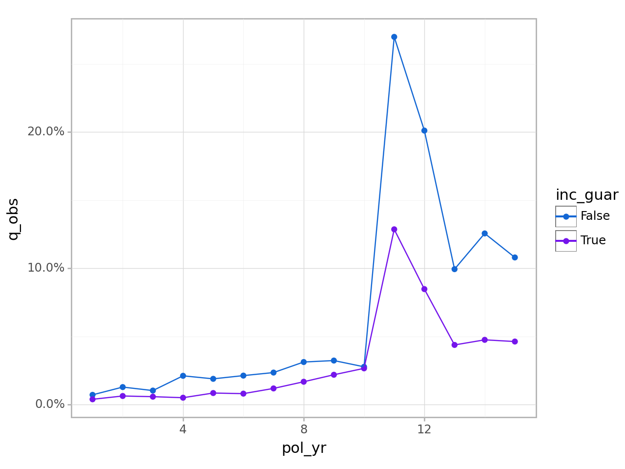
ExposedDF objects contain a group_by() method that is used to specify grouping variables for downstream methods like exp_stats(). Below, the data is grouped by policy year (pol_yr) and an indicator for the presence of a guaranteed income rider (inc_guar). After exp_stats() is called, the resulting output contains one record for each unique group.

exp_res = (exposed_data.
    group_by("pol_yr", "inc_guar").
    exp_stats())

exp_res
Experience study results

Groups: pol_yr, inc_guar
Target status: Surrender
Study range: 1900-01-01 to 2019-12-31

shape: (30, 6)
┌────────┬──────────┬──────────┬────────┬──────────────┬──────────┐
│ pol_yr ┆ inc_guar ┆ n_claims ┆ claims ┆ exposure     ┆ q_obs    │
│ ---    ┆ ---      ┆ ---      ┆ ---    ┆ ---          ┆ ---      │
│ u32    ┆ bool     ┆ u32      ┆ u32    ┆ f64          ┆ f64      │
╞════════╪══════════╪══════════╪════════╪══════════════╪══════════╡
│ 1      ┆ false    ┆ 56       ┆ 56     ┆ 7719.80545   ┆ 0.007254 │
│ 1      ┆ true     ┆ 46       ┆ 46     ┆ 11532.402336 ┆ 0.003989 │
│ 2      ┆ false    ┆ 92       ┆ 92     ┆ 7102.810869  ┆ 0.012953 │
│ 2      ┆ true     ┆ 68       ┆ 68     ┆ 10611.955805 ┆ 0.006408 │
│ 3      ┆ false    ┆ 67       ┆ 67     ┆ 6446.913856  ┆ 0.010393 │
│ …      ┆ …        ┆ …        ┆ …      ┆ …            ┆ …        │
│ 13     ┆ true     ┆ 49       ┆ 49     ┆ 1117.137361  ┆ 0.043862 │
│ 14     ┆ false    ┆ 33       ┆ 33     ┆ 262.622262   ┆ 0.125656 │
│ 14     ┆ true     ┆ 29       ┆ 29     ┆ 609.216476   ┆ 0.047602 │
│ 15     ┆ false    ┆ 8        ┆ 8      ┆ 74.046456    ┆ 0.10804  │
│ 15     ┆ true     ┆ 9        ┆ 9      ┆ 194.128602   ┆ 0.046361 │
└────────┴──────────┴──────────┴────────┴──────────────┴──────────┘

Actual-to-expected rates

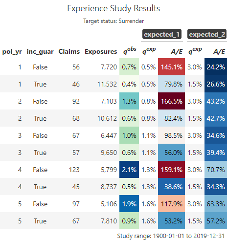
To derive actual-to-expected rates, first attach one or more columns of expected termination rates to the exposure data. Then, pass these column names to the expected argument of exp_stats().

expected_table = np.concatenate((np.linspace(0.005, 0.03, 10),
                                 [.2, .15], np.repeat(0.05, 3)))

# using 2 different expected termination rates
exposed_data.data = exposed_data.data.with_columns(
    expected_1=expected_table[exposed_data.data['pol_yr'] - 1],
    expected_2=pl.when(pl.col('inc_guar')).then(0.015).otherwise(0.03)
)

exp_res = (exposed_data.
           group_by("pol_yr", "inc_guar").
           exp_stats(expected=["expected_1", "expected_2"]))

exp_res
Experience study results

Groups: pol_yr, inc_guar
Target status: Surrender
Study range: 1900-01-01 to 2019-12-31
Expected values: expected_1, expected_2

shape: (30, 10)
┌────────┬──────────┬──────────┬────────┬───┬────────────┬────────────┬──────────────┬─────────────┐
│ pol_yr ┆ inc_guar ┆ n_claims ┆ claims ┆ … ┆ expected_1 ┆ expected_2 ┆ ae_expected_ ┆ ae_expected │
│ ---    ┆ ---      ┆ ---      ┆ ---    ┆   ┆ ---        ┆ ---        ┆ 1            ┆ _2          │
│ u32    ┆ bool     ┆ u32      ┆ u32    ┆   ┆ f64        ┆ f64        ┆ ---          ┆ ---         │
│        ┆          ┆          ┆        ┆   ┆            ┆            ┆ f64          ┆ f64         │
╞════════╪══════════╪══════════╪════════╪═══╪════════════╪════════════╪══════════════╪═════════════╡
│ 1      ┆ false    ┆ 56       ┆ 56     ┆ … ┆ 0.005      ┆ 0.03       ┆ 1.450814     ┆ 0.241802    │
│ 1      ┆ true     ┆ 46       ┆ 46     ┆ … ┆ 0.005      ┆ 0.015      ┆ 0.797752     ┆ 0.265917    │
│ 2      ┆ false    ┆ 92       ┆ 92     ┆ … ┆ 0.007778   ┆ 0.03       ┆ 1.665337     ┆ 0.431754    │
│ 2      ┆ true     ┆ 68       ┆ 68     ┆ … ┆ 0.007778   ┆ 0.015      ┆ 0.823869     ┆ 0.427191    │
│ 3      ┆ false    ┆ 67       ┆ 67     ┆ … ┆ 0.010556   ┆ 0.03       ┆ 0.984559     ┆ 0.346419    │
│ …      ┆ …        ┆ …        ┆ …      ┆ … ┆ …          ┆ …          ┆ …            ┆ …           │
│ 13     ┆ true     ┆ 49       ┆ 49     ┆ … ┆ 0.05       ┆ 0.015      ┆ 0.877242     ┆ 2.924141    │
│ 14     ┆ false    ┆ 33       ┆ 33     ┆ … ┆ 0.05       ┆ 0.03       ┆ 2.513115     ┆ 4.188525    │
│ 14     ┆ true     ┆ 29       ┆ 29     ┆ … ┆ 0.05       ┆ 0.015      ┆ 0.952043     ┆ 3.173475    │
│ 15     ┆ false    ┆ 8        ┆ 8      ┆ … ┆ 0.05       ┆ 0.03       ┆ 2.160806     ┆ 3.601343    │
│ 15     ┆ true     ┆ 9        ┆ 9      ┆ … ┆ 0.05       ┆ 0.015      ┆ 0.92722      ┆ 3.090735    │
└────────┴──────────┴──────────┴────────┴───┴────────────┴────────────┴──────────────┴─────────────┘

plot() and table() methods

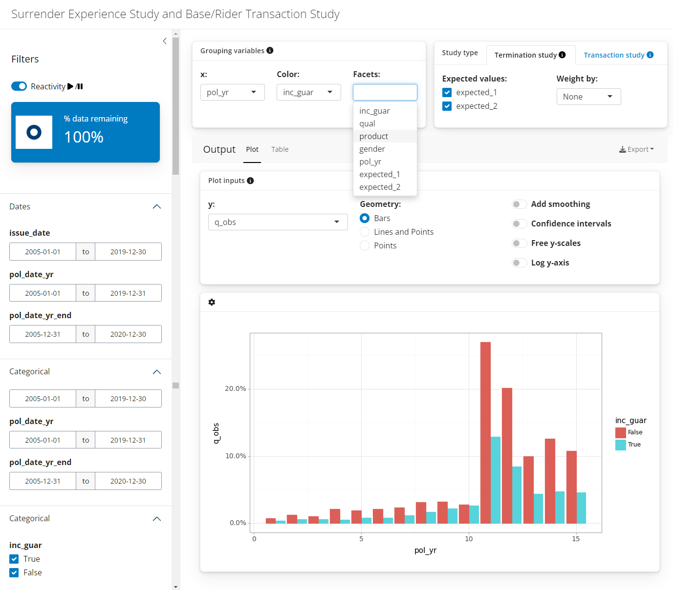
ExpStats objects have plot() and table() methods that create visualizations and summary tables. See Data visualizations for full details on these functions.

exp_res.plot()

<Figure Size: (640 x 480)>
# first 10 rows showed for brevity
exp_res.table()

summary()

Calling the summary() method on an ExpStats object re-summarizes experience results. This also produces an ExpStats object.

exp_res.summary()
Experience study results

Target status: Surrender
Study range: 1900-01-01 to 2019-12-31
Expected values: expected_1, expected_2

shape: (1, 8)
┌──────────┬────────┬─────────────┬──────────┬────────────┬────────────┬─────────────┬─────────────┐
│ n_claims ┆ claims ┆ exposure    ┆ q_obs    ┆ expected_1 ┆ expected_2 ┆ ae_expected ┆ ae_expected │
│ ---      ┆ ---    ┆ ---         ┆ ---      ┆ ---        ┆ ---        ┆ _1          ┆ _2          │
│ u32      ┆ u32    ┆ f64         ┆ f64      ┆ f64        ┆ f64        ┆ ---         ┆ ---         │
│          ┆        ┆             ┆          ┆            ┆            ┆ f64         ┆ f64         │
╞══════════╪════════╪═════════════╪══════════╪════════════╪════════════╪═════════════╪═════════════╡
│ 2869     ┆ 2869   ┆ 132633.9007 ┆ 0.021631 ┆ 0.024242   ┆ 0.020895   ┆ 0.892305    ┆ 1.035233    │
│          ┆        ┆ 56          ┆          ┆            ┆            ┆             ┆             │
└──────────┴────────┴─────────────┴──────────┴────────────┴────────────┴─────────────┴─────────────┘

If additional variables are passed to *by, these variables become groups in the re-summarized ExpStats object.

exp_res.summary('inc_guar')
Experience study results

Groups: inc_guar
Target status: Surrender
Study range: 1900-01-01 to 2019-12-31
Expected values: expected_1, expected_2

shape: (2, 9)
┌──────────┬──────────┬────────┬────────────┬───┬────────────┬────────────┬────────────┬───────────┐
│ inc_guar ┆ n_claims ┆ claims ┆ exposure   ┆ … ┆ expected_1 ┆ expected_2 ┆ ae_expecte ┆ ae_expect │
│ ---      ┆ ---      ┆ ---    ┆ ---        ┆   ┆ ---        ┆ ---        ┆ d_1        ┆ ed_2      │
│ bool     ┆ u32      ┆ u32    ┆ f64        ┆   ┆ f64        ┆ f64        ┆ ---        ┆ ---       │
│          ┆          ┆        ┆            ┆   ┆            ┆            ┆ f64        ┆ f64       │
╞══════════╪══════════╪════════╪════════════╪═══╪════════════╪════════════╪════════════╪═══════════╡
│ false    ┆ 1601     ┆ 1601   ┆ 52123.2158 ┆ … ┆ 0.023481   ┆ 0.03       ┆ 1.308099   ┆ 1.023856  │
│          ┆          ┆        ┆ 84         ┆   ┆            ┆            ┆            ┆           │
│ true     ┆ 1268     ┆ 1268   ┆ 80510.6848 ┆ … ┆ 0.024734   ┆ 0.015      ┆ 0.636752   ┆ 1.049964  │
│          ┆          ┆        ┆ 72         ┆   ┆            ┆            ┆            ┆           │
└──────────┴──────────┴────────┴────────────┴───┴────────────┴────────────┴────────────┴───────────┘

Shiny App

ExposedDF objects have an exp_shiny() method that launches a Shiny app to enable interactive exploration of experience data.

exposed_data.exp_shiny()